Sentiment Analysis has been around for a while. The basic idea revolves around measuring and classifying emotions (often boiled down to a single positive/negative measurement from -1.0 to 1.0) based on lexical analysis. Back a good few years ago, when Facebook and Whatsapp (don't exactly remember if this was before the merge) made it possible for you to download your text conversations en-masse, I immediately did so and was amazed at the amount of data I had accumulated and the possibilities of extracting insights about my life and the patterns therein. Unfortunately, it ended up as a post-it that was never really picked up.

Two weeks ago, I found myself with a free weekend. Downloading my data again, I had found almost exponential growth in the conversations I had been having online - for someone who prefers face-to-face communication over text, I now had almost 100,000 messages exchanged on Messenger alone, spanning over half a decade. The right kind of analysis could reveal how I had changed as a person, how my conversational partners have changed, whether I'm prone to cyclic behavior and emotional states, and so much more.

Starting with sentiment analysis, I had put off working on this for so long I expected there to be existing suites I could leverage. Libraries that could directly process and work with information collected about your online presence as well as standard suites of graphing and analytics that connected to them. Unfortunately, other than a few tutorials for sentiment analysis libraries, I couldn't really find any.

Faced with two options - building a general purpose library or directly solving the questions I wanted answers through direct scripting - (and I'm not proud of the fact that I usually choose the latter), I decided to go for the first one this time around. Converse was the result, and in it's current state it is a sentiment analysis and plotting library for Messenger in python. My primary objectives were ease of use - I wanted something that could come out of the box and provide useful graphs - and a high degree of configurability. I'll explain some of the issues, solutions and possible vectors for analysis later, but in standard reverse-sear fashion, let's start with how to use it.

§Install and Setup

pip install converse

That's it. Or, if you're the kind to prefer an isolated, fully configured system with a demo application and sample conversations,

docker pull hrishioa/converse

should do the trick.

If you're using the library directly from python, you'll also need to download the corpora for TextBlob, the sentiment analysis library we're using, as follows -

python -m textblob.download_corpora lite

Once you've got the library, you need to download your data from facebook.

Disclaimer: Now before you do so, let me confirm that converse is an offline library (the extremely paranoid can disable network connectivity on the docker container), and I don't retain (nor do I have any interest in) any of your information. The code is quite short and on github, where you can also find the dockerfile and sample conversations. That being said, it makes use of several large libraries for sentiment analysis, plotting and data management (primarily plotly, pandas and Textblob), and I take no responsibility for your data.

Here are a few guides on how to download your data, but here's a quick overview:

1. Facebook.com -> General Account Settings page -> Download a copy of your facebook data

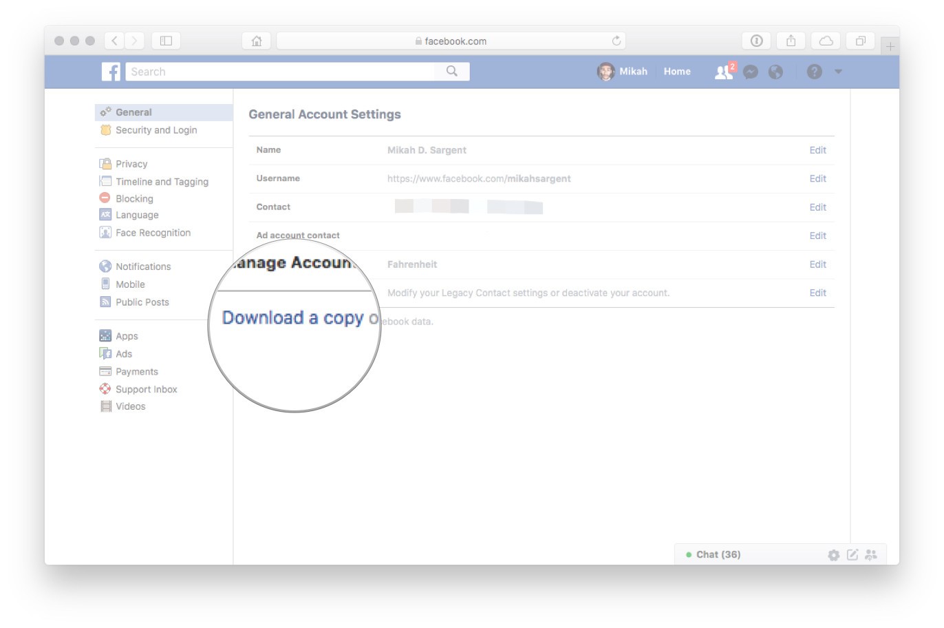
(Make sure to select JSON instead of HTML when choosing the format.)

2. Wait a while (possibly a few hours), before Facebook notifies you that your data is ready for download, and then grab it.
3. Unzip the archive to any directory you'd prefer. We're interested in the messages folder.

That's it. For the next step, run jupyter notebook where you'd like the code to live, and add the following code:

from converse import Conversation
from tqdm import tqdm_notebook as tqdm
from plotly.offline import init_notebook_mode, iplot

init_notebook_mode(connected=True)
convo = Conversation()
convo.load("path-to-message.json") # structure is usually archive-root/convo-name/message.json
iplot(convo.plot())

Replace path-to-message.json with the actual path to any conversation you'd like (the conversations are stored as a message.json file in folders marked by conversation names). Note that we're using Plotly's offline plotting library to keep things off the server.

And you should have a basic plot! Below is a sample plot of one of my conversations with the default settings:

The plot shows a single day moving average of the sentiment values of the conversation.

§Features

A full tutorial and demonstration of the features is part of the Docker image, and also in the github page here - Demo.ipnyb. I've removed the actual plots as they don't play well with github, and for anonymity reasons, but we can look at some of the more interesting features below.

§Time-based Moving Averages

The plot function accepts conventional time windows and multiple overlaid moving averages over the time window. For example, let's consider the same conversation shown above. The following will yield a daily chart, with 7, 30 and 365 SMAs:

iplot(convo.plot(timeframe="D", smas=[7,30,365]))

Or a weekly chart with a 1 and 4-week moving average:

iplot(convo.plot(timeframe="W", smas=[1,4]))

§OHLC Plotting

OHLC plotting was implemented, as one of my plans for future analysis included basic Technical and Harmonic Analysis, and can be turned on quite easily:

iplot(convo.plot(ohlc=True))

The colors can be customized as needed:

iplot(convo.plot(ohlc=True, ohlc_colors=['#00FF00','#FF0000']))

§Filters

The library also supports multiple conversations in the same object. Adding more conversations is as simple as using the load function, and each conversation is tagged by participant and title. As an example, loading all conversations into a single object can be done as follows using the glob library:

from glob import glob
for filename in glob('path-to-messages/*/message.json'):
	convo.load(filename)

Once this is done, the library supports immutable filters that can be chained for selecting particular ranges of data. The plots can also be overlaid using the + operator. Here's a complicated but readable example:

target_plot = allconvos \
    .filter_by_name("Target") \
    .filter_by_datetime(datetime(2017,7,14), datetime(2017,10,13)) \
    .plot(timeframe="W",smas=[4],label="Target")

everyone_else_plot = allconvos \
    .filter_by_name("Target", including=False) \
    .filter_by_datetime(datetime(2017,7,14), datetime(2017,10,13)) \
    .plot(timeframe="W",smas=[4],label="Everyone Else")

plot(target_plot+everyone_else_plot)

We can see that this particular friend of mine runs a lot happier in his conversations than the average :)

Here, we're plotting the weekly moving average for a single user against the total average of all the others I was talking to at the time, for a specific window. The docs should better illuminate how this works.

§Annotations and Density

The library also support density plots that show how many messages were aggregated into each average point. This can be helpful in explaining volatility (a point with 50 messages is likely to be less volatile than one with 2) and tracking conversational density.

iplot(convo.plot(timeframe="D",smas=[30],density=True))

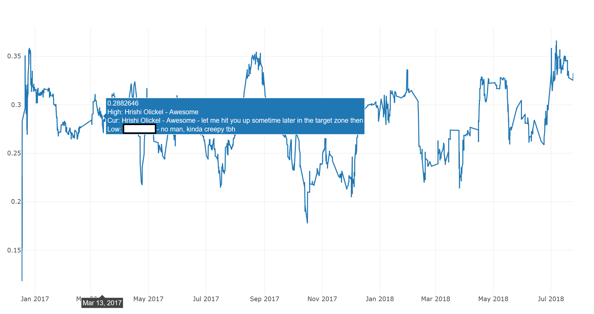
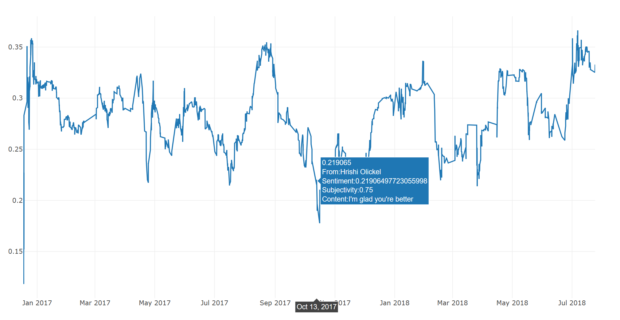
There are also annotation functions that can show exactly what a data point contains. The two provided ones, annot_highlow and annot_current_with_subjectivity, show different things (These plots are non-interactive, for the sake of privacy):

That's all for now. Next part (when I can get around to it) is using harmonic analysis to possibly track and predit cyclic behavior, as well as adding normalization functions to the library to better combat noise. I should mention again that this was a weekend project, so it's still extremely rough around the edges. Any and all feedback is welcome!

Hrishi Olickel

20 Jul 2018

hrishi[at]grey-wing.com