§Theory

§Background

In Computer Vision, Optical Flow deals with the detection of apparent movement between the frames of a video, or between images. The simplest of these is called a Lucas-Kanade Tracker, which attempts to solve the Optical Flow equation using the least-squares method.

§Method

The Optical-flow equation for Lucas-Kanade assumes that the change - or displacement - of moving objects between sucessive frames is small. This can be extended to fast-moving objects using other methods, and we will cover that in a separate post. Assuming small movement between frames, we end up with the following simple equation:

The proof can be found on wikipedia so I'm not going to go into detail. But in simple terms, $I_x$ and $I_y$ denotes intensity change in the x and y directions, and $V_x$ and $V_y$ stand for velocity, which we need to solve for. $I_t$ is the change in intensity w.r.t time (between frames).

If you're astute in math you will have noticed that this is a single equation in two unknowns ($V_x$ and $V_y$). In order to solve it, we need to introduce additional restrictions. In order to do that, we need to make assumptions about the data. At the basic level, different solutions make different assumptions to solve for different conditions.

§Lucas-Kanade Solution

Lucas-Kanade is one of the oldest solutions for the Optical Flow equation, and it assumes that the movement between successive frames is small and uniform within a the window being considered. If we do this, we can assume that the solution for the equation we saw before is the same for all these pixels. Namely,

Now, we have more equations than we have unknowns. Once again, the assumption of uniform velocity reduces the size of $V_x$ and $V_y$ to two variables for a small window. Now all we need are windows to look into.

§Corner Tracking

We need to identify points where motion can be detected in successive frames. It stands to reason that motion can be detected easily in corners, as there may not be enough detection in uniform areas within the tracked object.

The science of corner detection is almost as deep as that of optical flow, and the two often go hand in hand. For this implementation, as we're focusing on Optical Flow (and because of my inexperience), we're going to pick the simplest. Moravec Corner-Detection makes the assumption that a corner is a point of low self-similarity. There are many complex mathematical implementations of this, but we're simply looking for a few corners so we can see our algorithm in action. But before we do that, we need to set up.

§Implementation

§XCode

We're going to need some functionality for capturing and representing images. For this purpose, (and this purpose alone) we're going to use OpenCV. Later on - once this concept is stable - we can start using functions from OpenCV so we're not building on reinvented wheels.

Setting up OpenCV in XCode turned out to be relatively painless. There are two tutorials online that made this easy, one on installing OpenCV libraries on Mac, and the other on linking the installed libraries to XCode. Make sure the libraries are installed by running the following piece of code.

#include <opencv2/imgcodecs.hpp>
int main(int ac, char** av) {
    Mat img;
}

If it compiles and links fine, we're ready for implementation.

§Moravec Corner Detection

Implementation here is quite easy. Here's a simplified version of the full system:

deque<Point> findCorners(Mat img, int xarea, int yarea, int thres, bool verbose=true) {
        deque<Point> corners;

        ofstream log; //This will be used for dumping raw data for corner analysis
        log.open("log.csv");
        log << "x,y,score1,score2\n";

        //Image for marking up corners
        Mat outimg = img.clone();

        //Dimensions
        int dimx = img.cols, dimy = img.rows;

        //Count number of corners, start looping
        int count = 0;
        for(int startx=0;(startx+xarea)<dimx;startx+=xarea)
            for(int starty=0;(starty+yarea)<dimy;starty+=yarea)
            {
                count++;
                Mat curarea = img(Range(starty,min(starty+yarea,dimy)),Range(startx,min(dimx,startx+xarea)));
                double results[2] = {0,0};
                for(int dir = 0;dir<4;dir++)
                {
                    int newsx=startx,newsy=starty;
                    //Check similarity in each direction
                    switch(dir)
                    {
                        case 0: //left
                            newsx-=xarea;
                            newsx = max(newsx,0);
                            break;
                        case 1: //top
                            newsy-=yarea;
                            newsy = max(newsy,0);
                            break;
                        case 2: //right
                            newsx+=xarea;
                            newsx = min(newsx,dimx);
                            break;
                        case 3: //down
                            newsy+=yarea;
                            newsy = min(newsy,dimy);
                            break;
                        default:
                            break;
                    }
                    Mat newarea = img(Range(newsy,min(newsy+yarea,dimy)),Range(newsx,min(newsx+xarea,dimx)));

                    if(newarea.cols!=curarea.cols || newarea.rows!=curarea.rows)
                        continue;

                    Mat diff = abs(curarea-newarea);
                    results[dir%2] = mean(mean(diff))(0);
                }
                results[0]/=2;
                results[1]/=2;

                //thresholding
                if(results[0]>=thres && results[1]>=thres)
                {
                    corners.push_back(Point(startx,starty));
                    rectangle(outimg, Point(startx,starty), Point(startx+xarea,starty+yarea), Scalar(0),2);
                }

                log << startx << "," << starty << "," << results[0] << "," << results[1] << "\n";
            }
        log.close();
        return corners;
    }
}

We're isolating windows, looking at equal sized windows in each direction, and compiling a score that would tell us the probability of a particular window containing a corner. We're also taking into account the size of the image and any possible issues we could have with clipping.

It really shows how rusty my C++ is. There are many optimizations we can make. The simplest one would be to detect anomalies using larger windows, and zoom in using the same method to the required window size. This would cut down on the number of windows we need to analyze before we're done. Also, there is a better way of corner detection that doesn't depend on cardinal directions (north, south, east, west) for identificaton. However, there are already built and optimized state-of-the-art algorithms in the OpenCV library that we can use. For simplicity, we're going to keep corner detection as it is.

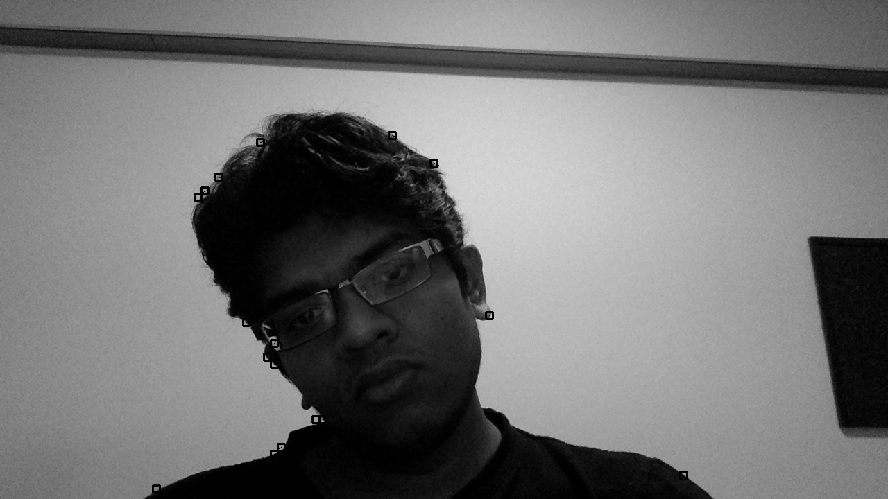
Looking at the results, we've managed to isolate a few useful markers to track motion:

##Lucas-Kanade Corner Tracking

Remember the equation we considered before:

,

,

$Av = T$

We can solve for v:

$v = A^{-1}T$

And here we can see why we're looking for corners. The matrix $A$ needs to be inversible, and by selecting corners we exclude the uniform areas of the image that would prevent this.

First, we compute $I_x$ and $I_y$ for each pixel using the intensity values of adjacent pixels:

Ix.at<uchar>(y,x) = ((int)imgA.at<uchar>(y,px)-(int)imgA.at<uchar>(y,nx))/2;
Iy.at<uchar>(y,x) = ((int)imgA.at<uchar>(py,x)-(int)imgA.at<uchar>(ny,x))/2;

Computing $I_t$ by subtracting intensity values between frames:

double curdI = ((int)imgA.at<uchar>(y,x)-(int)imgB.at<uchar>(y,x));

And here is the part I'm ashamed of. I was working with a vanilla install of XCode, and not wanting to bother with matrix libraries, I decided to implement it by hand:

double detG = (G[0][0]*G[1][1])-(G[0][1]*G[1][0]);
double Ginv[2][2] = {0,0,0,0};
Ginv[0][0] = G[1][1]/detG;
Ginv[0][1] = -G[0][1]/detG;
Ginv[1][0] = -G[1][0]/detG;
Ginv[1][1] = G[0][0]/detG;

But it works, and final implementation shows both the corners and the velocity values we've computed.

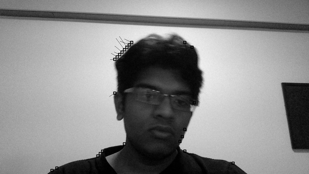
This is an intermediate step, and it serves to illustrate the underlying concept behind Lucas-Kanade. Next we'll move on to Horn-Shunck and eventually arrive at a more application-specific solution.

The complete working implementation can be found here.

Hrishi Olickel

5 Oct 2015

hrishi[at]grey-wing.com